
Bundestagswahl 2025: Offenbach by Wahlbezirk
Published:
Offenbach has voted. Here’s how the 79 polling districts (Wahlbezirke) went, mapped by Zweitstimme (second vote) winner. The 24 postal voting districts are excluded.
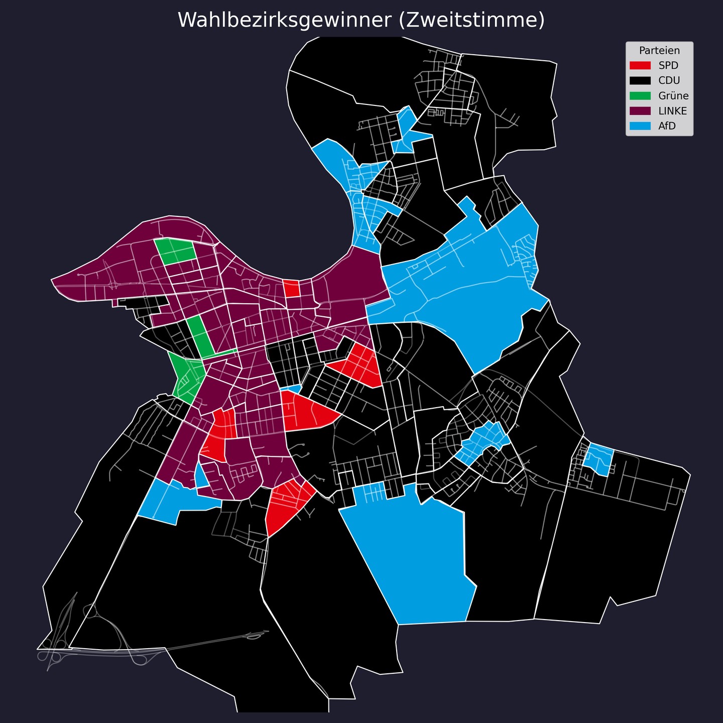
District-level winners: CDU 31, Linke 30, AfD 10, SPD 5, Grüne 3.
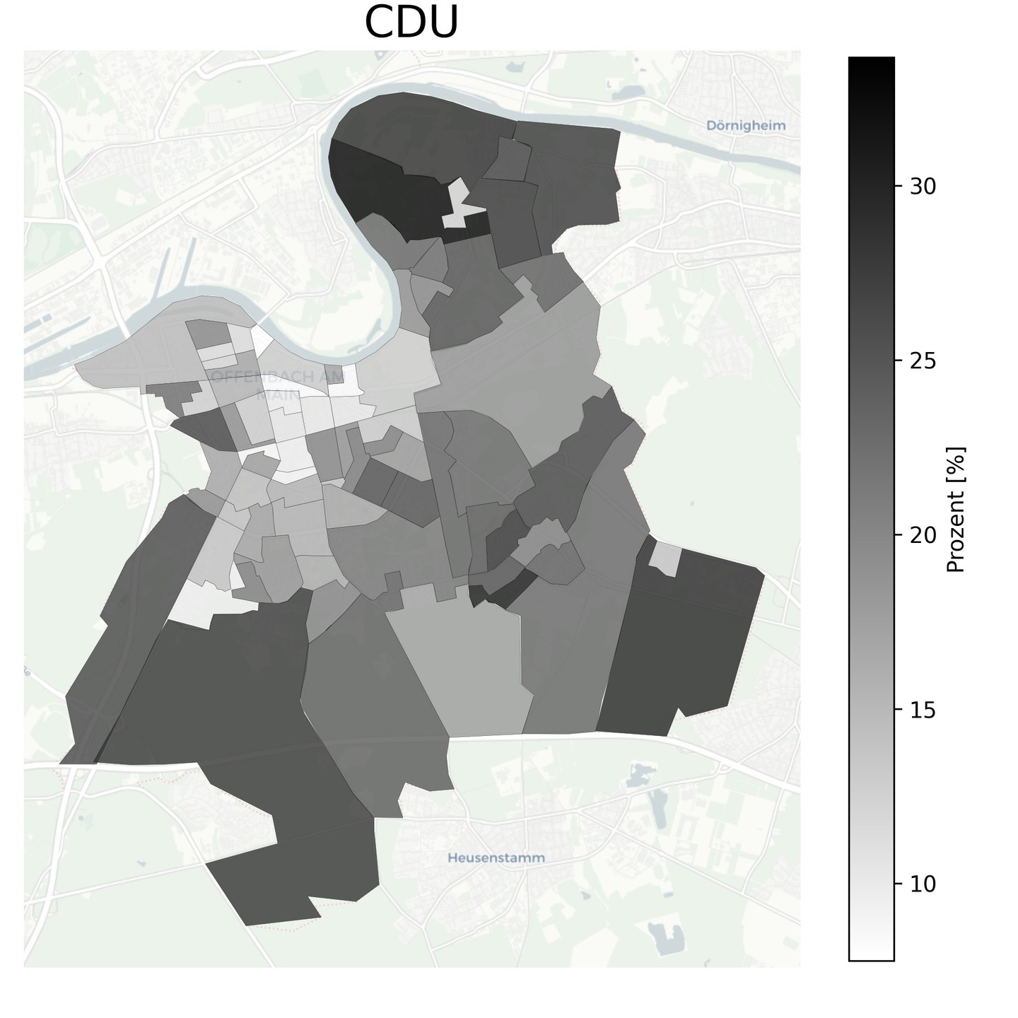
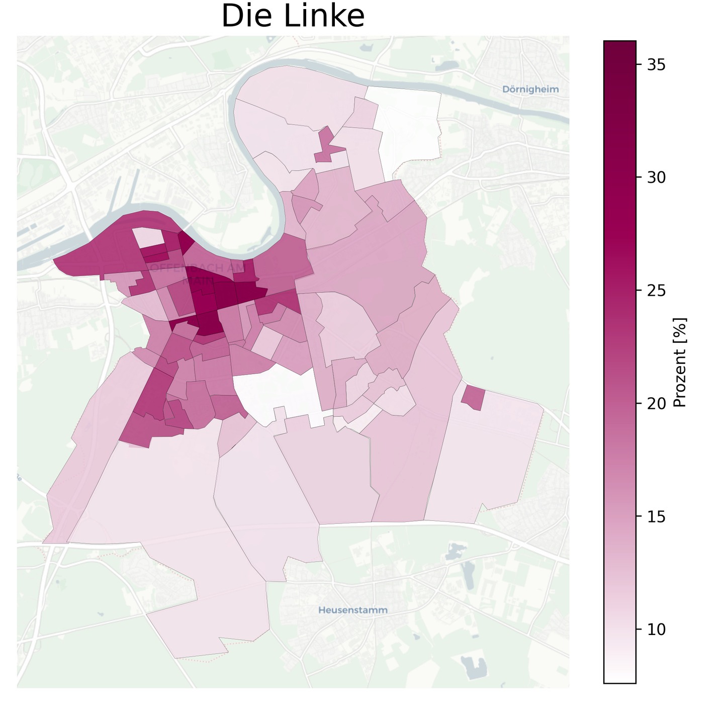
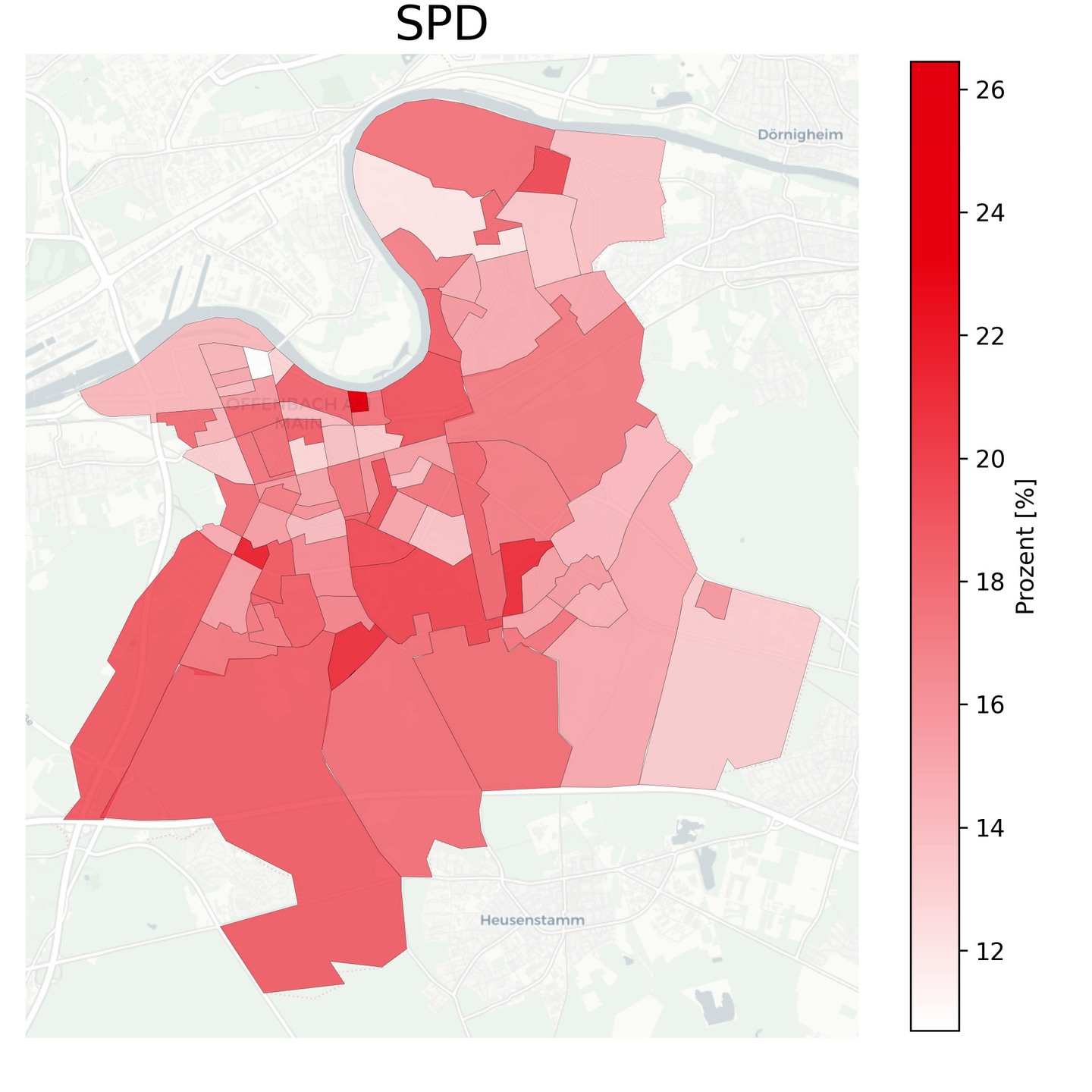
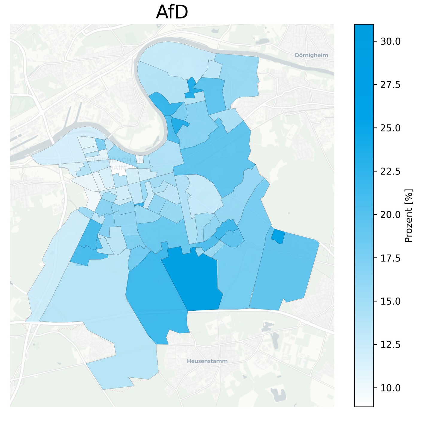
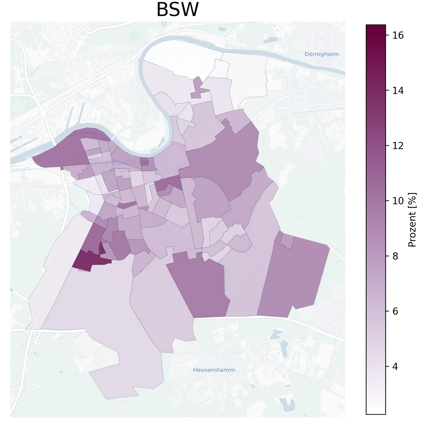
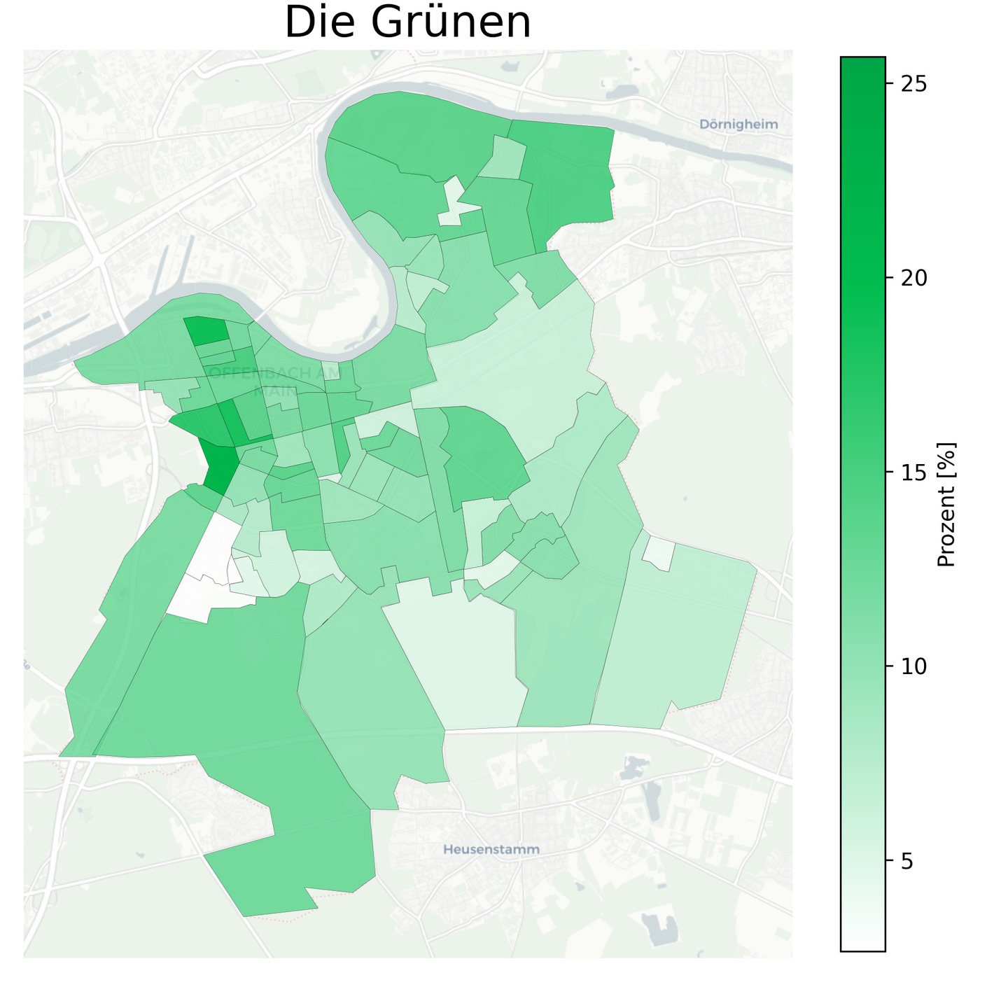
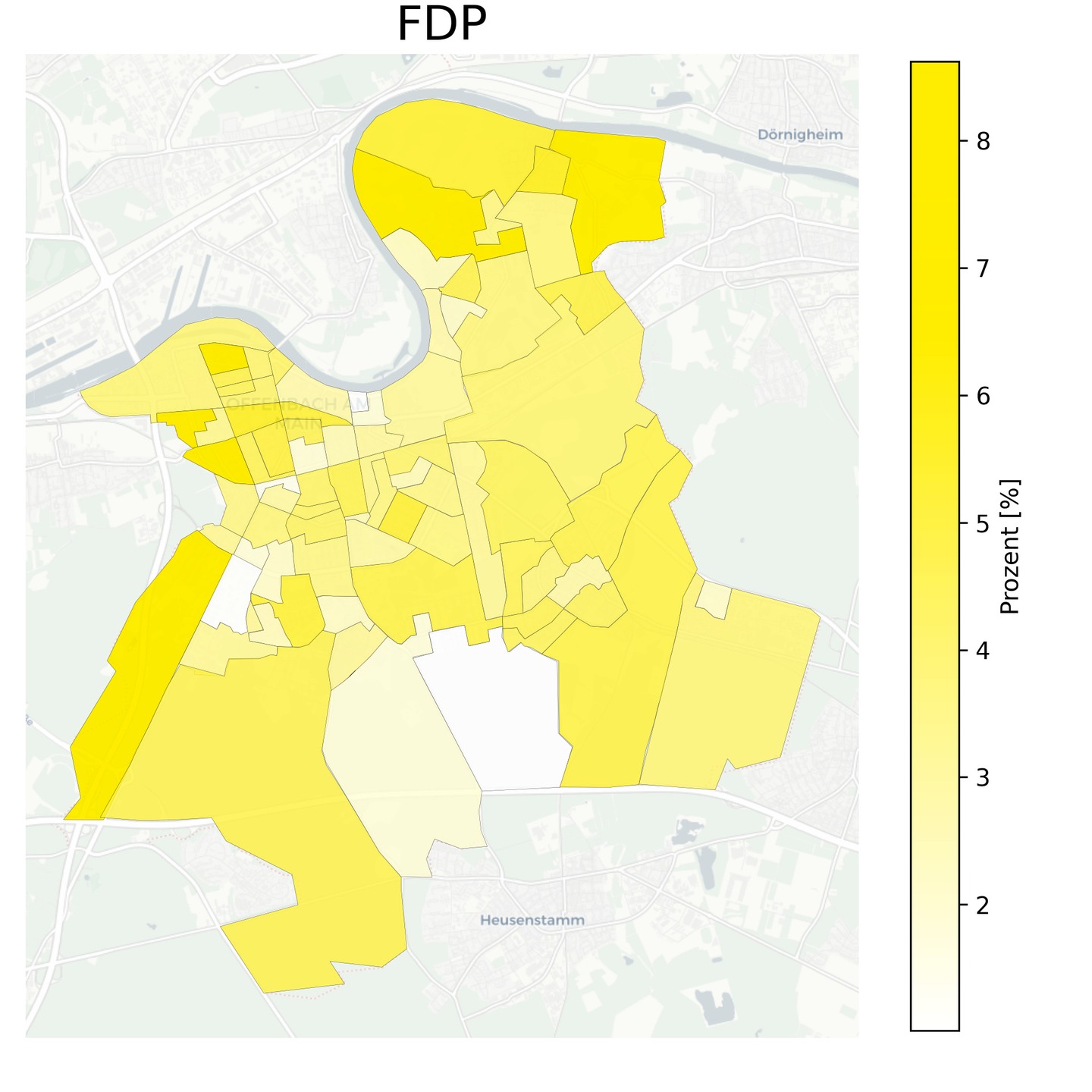
The remaining charts show the geographic distribution of Zweitstimme shares per party:
Data and code
Election results from Votemanager Open Data (Stand 24.02.2025, 09:00). Wahlbezirk geometries via GeoJSON (props to @lsy_161).
import geopandas as gpd
import pandas as pd
import matplotlib.pyplot as plt
import osmnx as nx
import contextily as cx

# Load Wahlbezirk geometries and election results
gdf = gpd.read_file("wahlbezirke.geojson")
wahl_df = pd.read_csv("data/Open-Data-06413000-Bundestagswahl-Wahlbezirk.csv", sep=";")
wahl_df.rename(columns={"gebiet-nr": "Wahlbezirk"}, inplace=True)

# Merge, keep Zweitstimmen columns (F1, F2, ...)
df = gdf.merge(wahl_df, on="Wahlbezirk")
zweitstimmen_cols = [c for c in df.columns if c.startswith("F") and c != "F"]
df_filtered = df[["Wahlbezirk", "geometry"] + zweitstimmen_cols]

# Winner per district = column with max Zweitstimmen
max_values = df_filtered.loc[:, zweitstimmen_cols].idxmax(axis=1)

# Plot each district with party color (F1=SPD, F2=CDU, F6=Linke, etc.)
fig, ax = plt.subplots(figsize=(12, 12))
for i, mv in enumerate(max_values):
    df_filtered.loc[[i], "geometry"].plot(ax=ax, color=parteifarben[mv], alpha=1., edgecolor="#ffffff")
cx.add_basemap(ax, crs=df_filtered.crs, source=nx.providers.OpenStreetMap.Mapnik)
OSM base map via OSMnx and contextily. Full notebook: bundestagswahl2025.ipynb.