
Isochrone Maps with Python
Published:
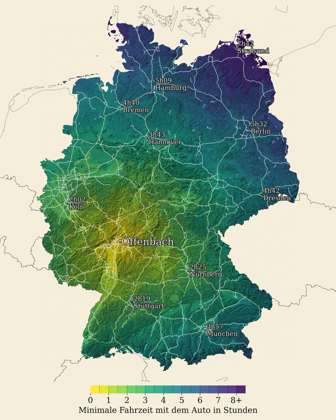
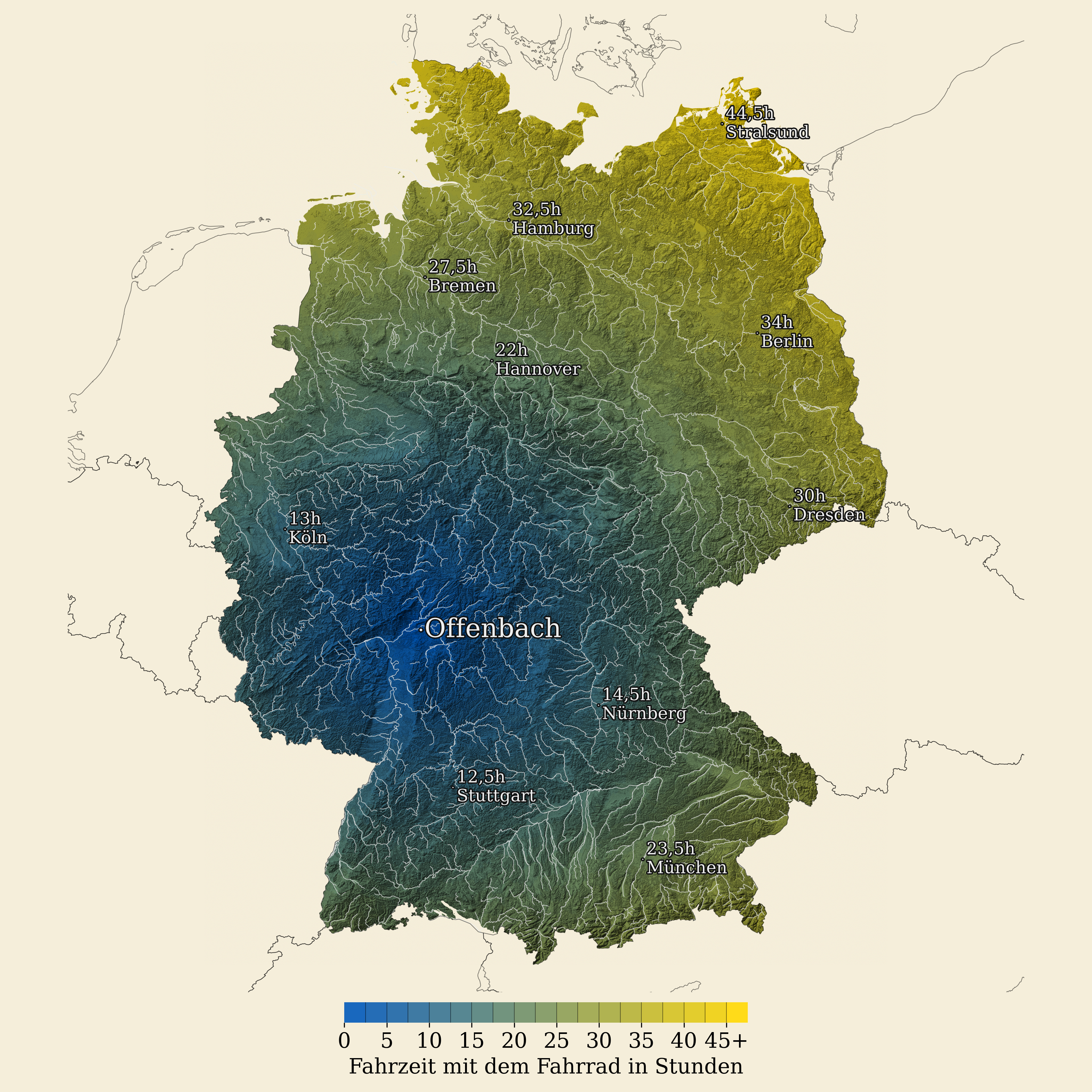
Isochrone maps show areas reachable within a given travel time from a starting point. This project combines OSRM travel time calculations with satellite-derived elevation data to produce maps that show both accessibility and topography.
Process overview
- Load and process a Digital Elevation Model (DEM)
- Calculate travel times via OSRM
- Color-code administrative areas by travel time
- Overlay hillshading, city labels, and street networks
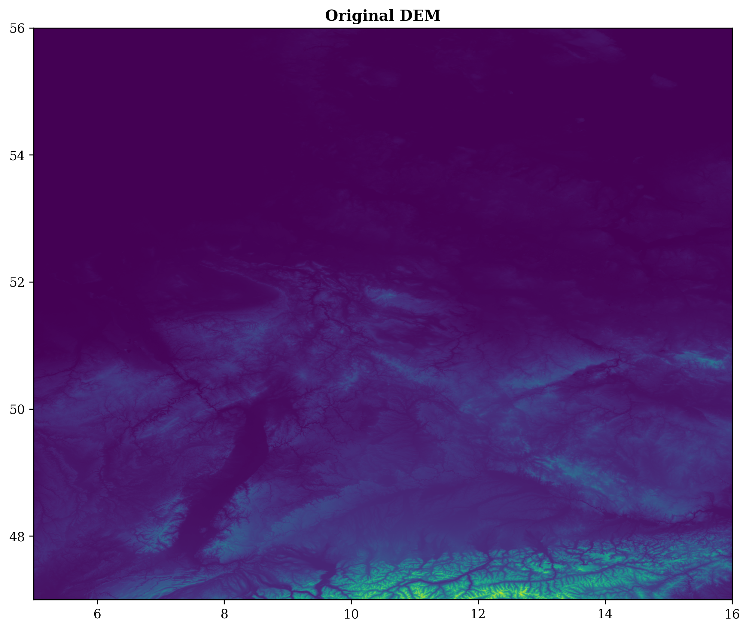
DEM processing
The elevation data goes through several steps: CRS transformation, masking to the area of interest, and hillshading.
def _process_dem(self):
    if self.kwargs.use_elevation:
        bounds = self.get_shp_bounds()
        elevation_file = self.get_elevation_dem(bounds)
    else:
        elevation_file = self.kwargs.dem_file

    with rio.open(elevation_file) as src:
        working_dem = transform_dem(src, self.config["dem"]["dest_crs"])
        if self.kwargs.reduce_size != 1.0:
            working_dem = resize_dem(working_dem, self.kwargs.reduce_size)
        working_dem = mask_dem(working_dem, self.admin_shp["geometry"])
        transformed_shaded = hillshade(working_dem.read(1), azimuth=315, angle_altitude=45)
        return recreate_dataset_reader(transformed_shaded, working_dem.meta, 1)
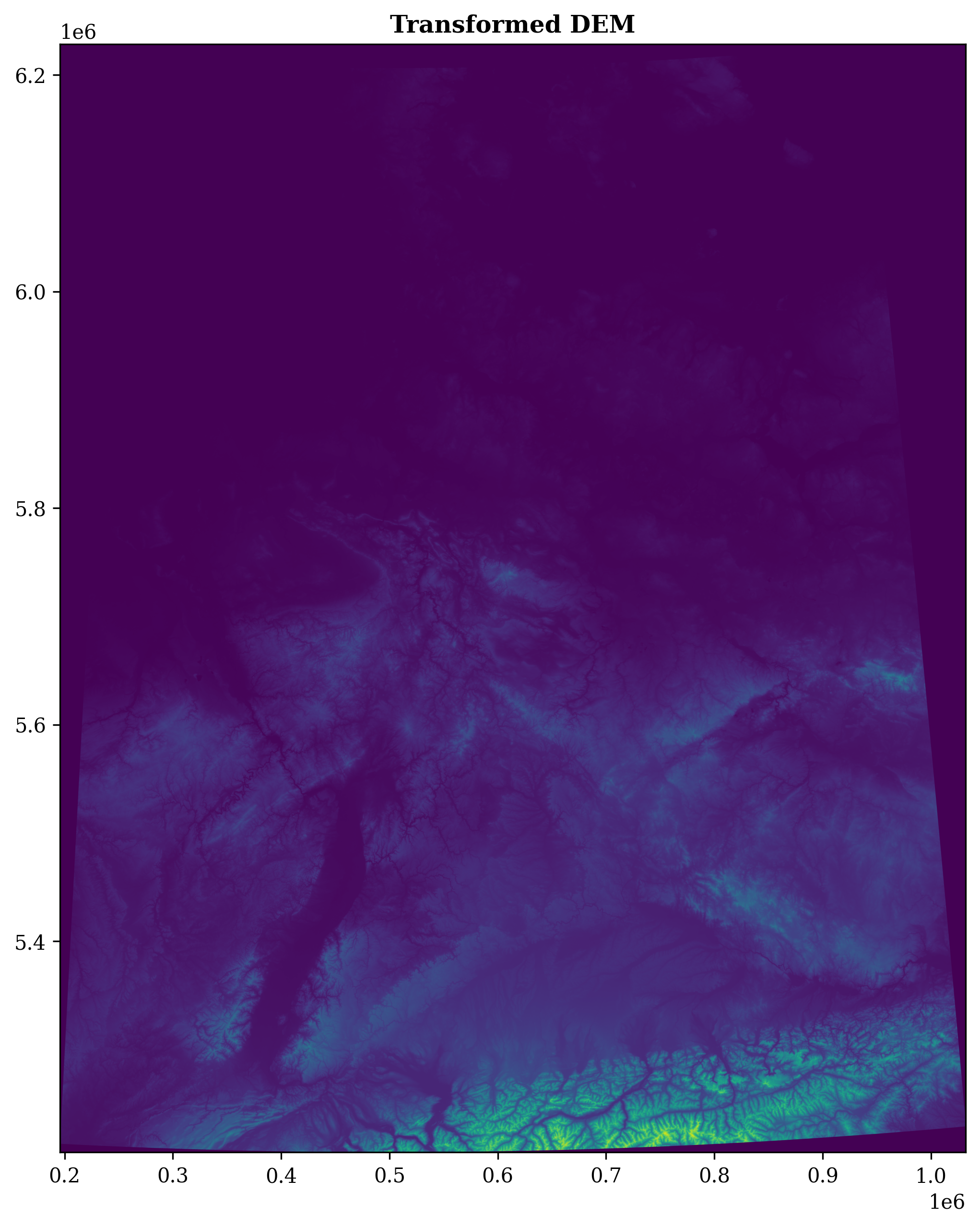
CRS transformation is straightforward with rasterio:
def transform_dem(dem_dataset, target_crs):
    if dem_dataset.crs == target_crs:
        return dem_dataset
    transform, width, height = calculate_default_transform(
        dem_dataset.crs, target_crs,
        dem_dataset.width, dem_dataset.height,
        *dem_dataset.bounds
    )
    kwargs = dem_dataset.meta.copy()
    kwargs.update({'crs': target_crs, 'transform': transform, 'width': width, 'height': height})
    return recreate_dataset_reader(dem_dataset.read(), kwargs)
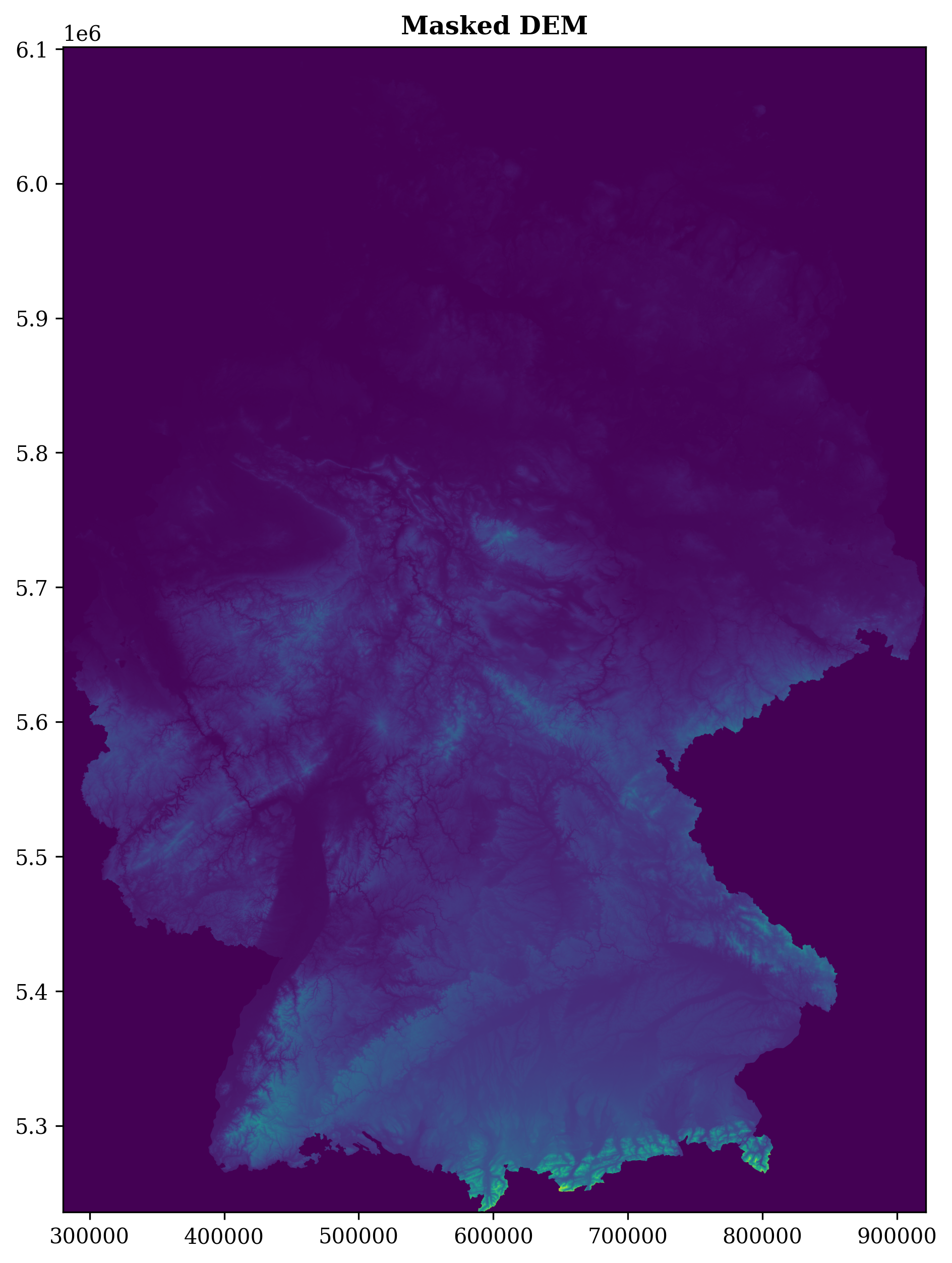
Masking clips the raster to the administrative boundary:
def mask_dem(dem_dataset, geometries):
    out_image, out_transform = rio_mask(dem_dataset, geometries, crop=True, all_touched=True)
    out_meta = dem_dataset.meta.copy()
    out_meta.update({
        "height": out_image.shape[1], "width": out_image.shape[2], "transform": out_transform
    })
    return recreate_dataset_reader(out_image, out_meta)
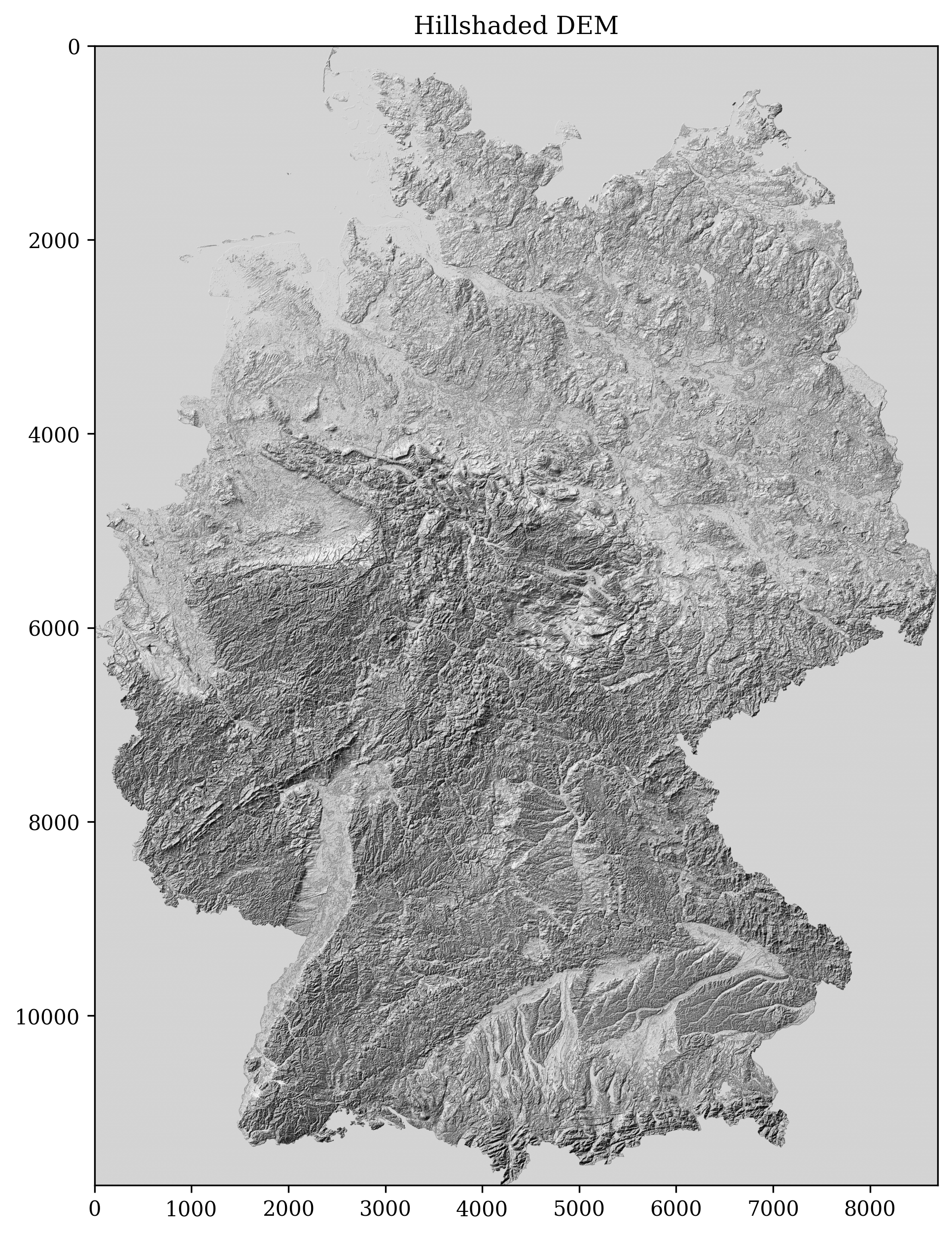
Hillshading uses gradient-based slope and aspect calculation:
def hillshade(array, azimuth=315, angle_altitude=45):
    x, y = np.gradient(array)
    slope = np.pi/2 - np.arctan(np.sqrt(x*x + y*y))
    aspect = np.arctan2(-x, y)
    azimuthrad = azimuth * np.pi / 180
    altituderad = angle_altitude * np.pi / 180
    return (np.sin(altituderad) * np.sin(slope) +
            np.cos(altituderad) * np.cos(slope) *
            np.cos((azimuthrad - np.pi/2) - aspect)) * 255
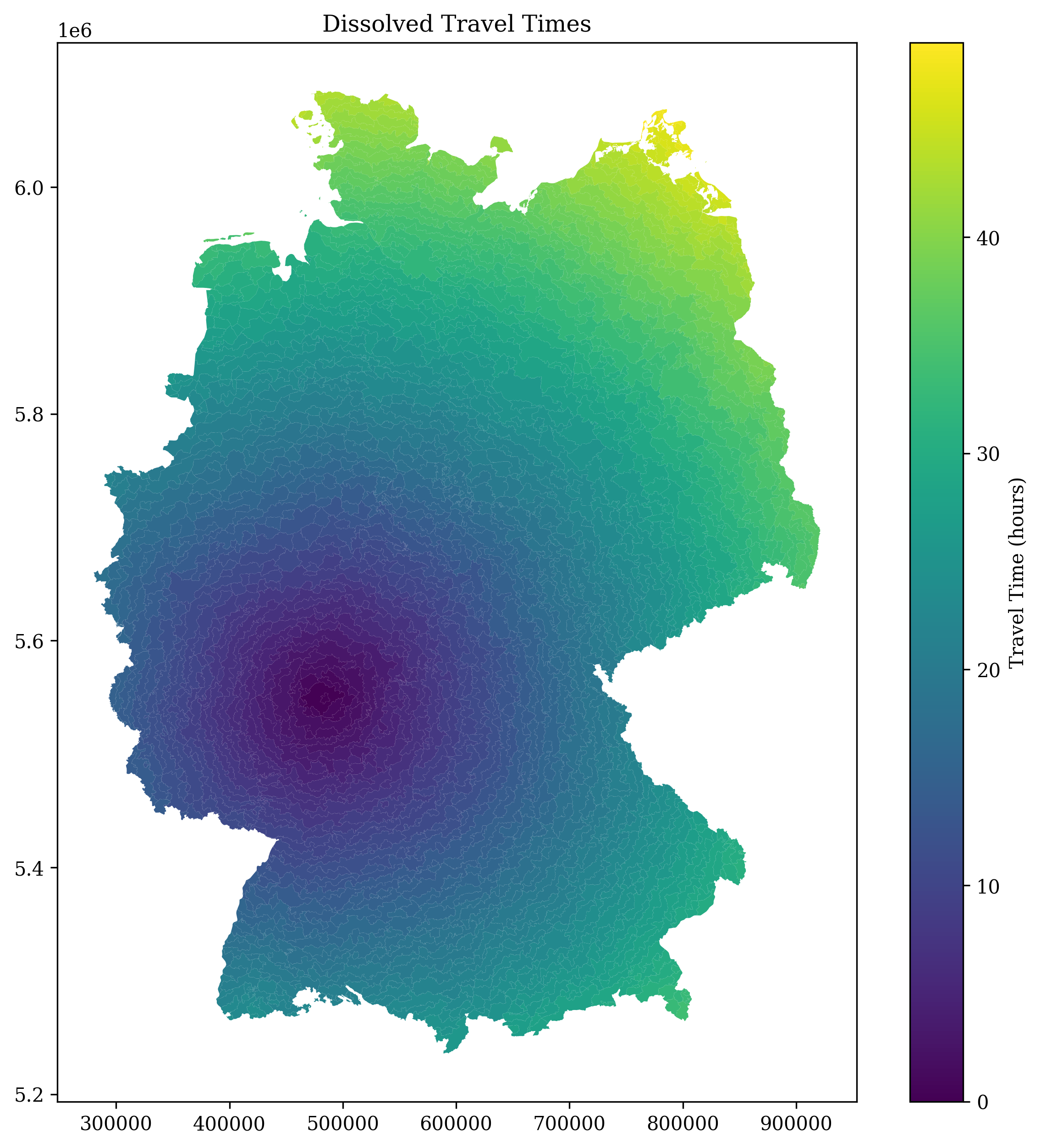
Travel time calculation
OSRM (Open Source Routing Machine) computes driving times from a central point to the centroid of every administrative area. Coordinates are converted from UTM to WGS84 before querying:

class OSRM:
    def calculate_travel_time(self, gdf):
        gdf = self._init_gdf_fields(gdf)
        for _, row in tqdm(gdf.iterrows(), total=len(gdf)):
            utm_x, utm_y = row["geometry"].centroid.coords[0]
            lat, lon = utm.to_latlon(utm_x, utm_y, 32, 'U')
            result = self._get_distance_duration(lat, lon)
            if result:
                distance, duration = result
                gdf = self._update_gdf(gdf, row["DEBKG_ID"], lat, lon, distance, duration)
        return gdf
The areas are then dissolved by travel time bucket for a cleaner visualization:
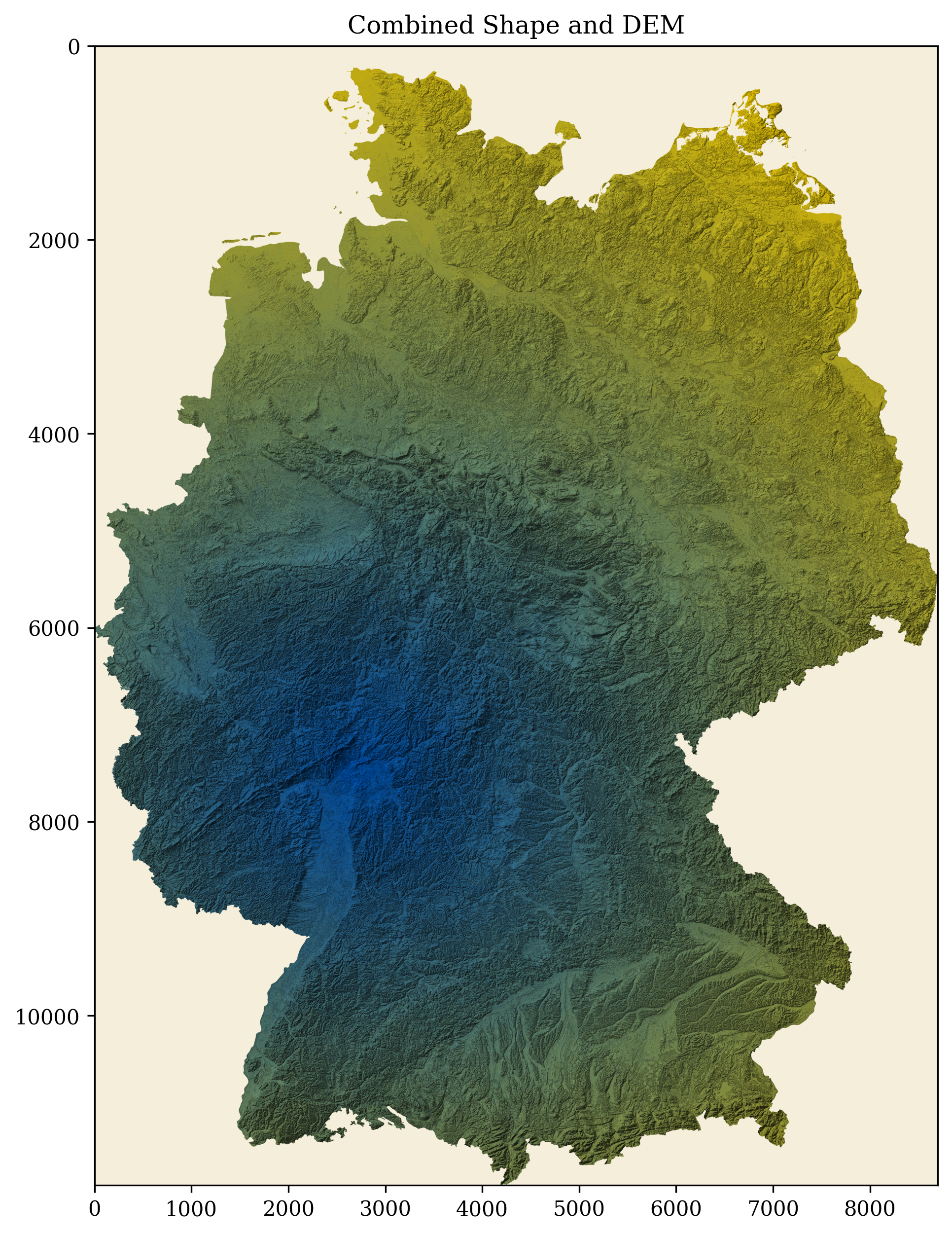
Combining DEM and travel times
Each administrative area is colored by travel time using a gold-to-blue gradient, then multiplied with the hillshade raster:
def combine_shape_dem(self, admin_gdf, dem):
    unique_colors = len(admin_gdf["traveltime_h"].unique())
    cmap = LinearSegmentedColormap.from_list(
        "Custom", [(255/255, 215/255, 0/255), (0/255, 87/255, 183/255)], N=unique_colors
    )
    base_image = np.full((dem.shape[0], dem.shape[1], 3), np.array([0, 0, 0]))

    for _, area in tqdm(admin_gdf.iterrows(), total=len(admin_gdf)):
        out_image, _ = rio_mask(dem, [area["geometry"]], crop=False, all_touched=False)
        color_index, ccode = self._get_colorcode_val(
            area["traveltime_h"], area["traveltime_h30"], unique_colors
        )
        rgba = cmap(ccode)
        rgb = np.array(rgba[:3])
        base_color = np.full((dem.shape[0], dem.shape[1], 3), rgb)
        image_data = np.expand_dims(out_image[0, :, :], axis=2)
        base_image = base_image + np.rint(base_color * image_data).astype("int")
    return base_image
Final map
The final render adds city labels, a street network overlay, and a legend:
def plot_map(colored_image, street_graph_edges, city_label_gdf, eu_gdf, config, legend_used_colors):
    fig, ax = plt.subplots(figsize=config["map"]["size"])
    ax.imshow(colored_image)
    if street_graph_edges is not None:
        street_graph_edges.plot(ax=ax, linewidth=0.5, alpha=0.5)
    for idx, row in city_label_gdf.iterrows():
        ax.annotate(row['city'], (row.geometry.x, row.geometry.y), fontsize=config["map"]["fontsize"])
    plot_legend(ax, legend_used_colors)
    plt.savefig(config["map"]["output_file"], dpi=300, bbox_inches='tight')
The coordinate handling juggles WGS84 (EPSG:4326) for GPS coordinates and UTM Zone 32N (EPSG:25832) for local measurements, with rasterio and GeoPandas handling the conversions.